HLookup function of Formulas tab in Microsoft Excel 2016

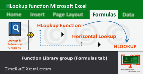
HLookup function of Lookup & Reference MS Excel

Hlookup Formula | Hlookup in Excel | Hlookup Function | Hlookup and Vlookup

Previous Post: VLookup function Lookup & Reference Microsoft Excel 2016

Alright, the previous post was on the VLookup function of the Formulas tab. Basically, this function helps us to retrieve answers referring from a column of a Table. Particularly, this table is in the Vertical direction. In fact, “V” is for Vertical, hence it is VLookup.

In the first place, the Full Form of HLookup is Horizontal Lookup. There could be various occasions, when users require to get their results, from a column of a Table. And, generally a table is in the Vertical direction, most often times. However, this type of table is best suited for the VLookup function.

But, according to this post and the HLookup function, the table orientation is in the Horizontal direction. Whereas, now the answers will get retrieved from the row, instead of a column. And, this is because of the direction of the table, the column becomes the row.

HLookup function of Formulas tab MS Excel – continued

To enumerate, here is a further explanation about on the HLookup Function. For example, we have two Tables, one of three columns on the Left Hand Side in worksheet. And, the other table has two Rows, and we need to get the answer from the second row from this table.

In fact, let us see what is the Syntax of the HLookup function. Also, to know about, what is a Syntax, users can refer to the previous post.

Syntax: HLOOKUP(lookup_value,table_array,col_index_num,[range_lookup])

So, now let know how to use the above mentioned HLookup function. The Lookup Value is the cell having the value on the left side of column. This is just adjacent to the right column that is empty.

Then, the Table Array, is the table from which users need get their result. Next, the Column Index Number in this case, for HLookup, is the second Row of the Table Array in selection.

HLookup function of Formulas tab Excel 2016

Moreover, the Range Lookup has further two options i.e. TRUE or FALSE. The True stands for Approximate Match and False is for Exact Match. We can choose either one option out of two mentioned. And, based on the selection, users get their answers, for the Column Index Number value.

Finally, to add, users need to sort the Row of the Table Array. Doing this will help to get correct answer which’re numerical data based. All together, the HLookup Function is not in much use; but is an important function in comparison to the VLookup function.

See Next Post: Left function Text functions Formulas tab Microsoft Excel 2016

Tags: Microsoft Excel Functions