Create Charts from data of worksheet Microsoft Excel 2016

Create Charts from data of worksheet MS Excel

Create Charts content worksheet Microsoft Excel

See Previous Post: Add Pictures Insert Images worksheet Microsoft Excel 2016

Significantly, in this post, we’ll discuss about how to Create Charts. The Insert tab ribbon has the Charts group. And, this group contains various chart buttons. Some of them are the Column or Bar Chart, Waterfall or Stock Chart and the PivotChart buttons etc; and so on.

Also, in one of the posts, all the buttons of the Charts group have been explained. But, it wasn’t about, how to create charts from the data in worksheet. Hence, we should know creating charts, as it’s important while learning in Microsoft Excel.

Create Charts from data Microsoft Excel – continued

Especially, the Charts are the graphical representation of a data. Also, comparison is done with the help of charts. And, this helps to know growth or downfall from the data. In addition, the Charts are quick way to project a comparison of the data from time to time. Whether it’s a Global Company or a Small Business, everybody needs it.

Suppose, we’ve a tabular type of data in a Excel sheet, of our virtual company. And, a chart has to be created from that data. So, let us know how to do that.

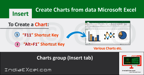
• First of all, select the tabular data.
• Then, press the Shortcut Key i.e. F11 or “Alt+F1“.
• And, the Chart from the data in selection gets created.

Most noteworthy, when the chart has been created, the Chart Tools tab will show up. It is found on the Upper Top of the Microsoft Excel window. Also, this tab has two other tabs within it. They’re the Design tab and the Format tab respectively.

Create Charts from data spreadsheet MS Excel 2016

The Design tab of the Chart Tools further shows multiple options for the Chart Designs. The users might choose the colorful charts designs that suits best according to the data. And, the Format tab helps to Insert Shapes, Shape Styles and the WordArt Styles etc; and so on for the Charts.

Lastly, while using the “F11” key for creating the chart; a separate sheet named “Chart1” on the Left side of the Sheet1 is created. And, the “Alt+F1” Shortcut Keys creates the chart in the same sheet which has the data.

See Next Post: Use Apply Conditional Formatting worksheet Microsoft Excel 2016

Tags: Microsoft Excel Buttons