IndiaExcel – Learn Microsoft Excel

Category: Microsoft Excel Buttons

  • Use Apply Conditional Formatting in worksheet MS Excel

    How to Use Apply Conditional Formatting MS Excel

    Use Apply Conditional Formatting worksheet MS Excel 2016
    Use Apply Conditional Formatting Microsoft Excel

    See Previous Post: Create Charts from data worksheet Microsoft Excel 2016

    As we know that, the Styles group has the Conditional Formatting button. So, we’ll know How to Use Apply Conditional Formatting in a worksheet, in this post. This button has total Eight buttons. Some of them’re the Highlight Cell Rules button, the Data Bars button and the Icon Sets button etc; and so on.

    Also, in one of the posts, we firstly got to know about the Conditional Formatting buttons. But, through this post, we’ll now know, how to use and apply them. Especially, the Conditional Formatting feature is quite captivating and attractive in terms of the functionality in Excel.

    Because, the Conditional Formatting helps users to distinguish between the data in worksheet. In addition, also users can highlight necessary aspects in the data using these various buttons. So, to apply the Conditional Formatting in a cell or multiple cells, these steps’re required. We’re taking an example of some random numbers present in a column.

    Use Apply Conditional Formatting MS Excel – continued

    • First of all, select the Column, Row or the Range of Cells which have numbers.
    • Then, go to the Highlight Cell Rules and select Greater Than button.
    • A Greater than dialog show up.
    • Now, type the number in the Text Box under Format cells that are GREATER THAN.
    • Next, select the color from the Combo Box on the right side of the Text Box.
    • And, finally click the OK button to Use and Apply the Conditional Formatting Rule.

    Similarly, the other buttons such as the Less Than button or the Text that Contains button etc; and so on, functions on the same process. But, the New Rule button, the Clear Rules button and the Manage Rules button works slightly different.

    Above all, also the Quick Analysis introduced in Microsoft Excel 2013 and Microsoft Excel 2016; helps to quickly and easily apply some of the types of Conditional Formatting rules. The Shortcut Key for the Quick Analysis tool is “Ctrl+Q“.

    See Next Post: Understand Fill Handle worksheet Microsoft Excel 2016

  • Create Charts from data of worksheet Microsoft Excel 2016

    Create Charts from data of worksheet MS Excel

    Create Charts content worksheet Microsoft Excel 2016
    Create Charts content worksheet Microsoft Excel

    See Previous Post: Add Pictures Insert Images worksheet Microsoft Excel 2016

    Significantly, in this post, we’ll discuss about how to Create Charts. The Insert tab ribbon has the Charts group. And, this group contains various chart buttons. Some of them are the Column or Bar ChartWaterfall or Stock Chart and the PivotChart buttons etc; and so on.

    Also, in one of the posts, all the buttons of the Charts group have been explained. But, it wasn’t about, how to create charts from the data in worksheet. Hence, we should know creating charts, as it’s important while learning in Microsoft Excel.

    Create Charts from data Microsoft Excel – continued

    Especially, the Charts are the graphical representation of a data. Also, comparison is done with the help of charts. And, this helps to know growth or downfall from the data. In addition, the Charts are quick way to project a comparison of the data from time to time. Whether it’s a Global Company or a Small Business, everybody needs it.

    Suppose, we’ve a tabular type of data in a Excel sheet, of our virtual company. And, a chart has to be created from that data. So, let us know how to do that.

    • First of all, select the tabular data.
    • Then, press the Shortcut Key i.e. F11 or “Alt+F1“.
    • And, the Chart from the data in selection gets created.

    Most noteworthy, when the chart has been created, the Chart Tools tab will show up. It is found on the Upper Top of the Microsoft Excel window. Also, this tab has two other tabs within it. They’re the Design tab and the Format tab respectively.

    Create Charts from data spreadsheet MS Excel 2016

    The Design tab of the Chart Tools further shows multiple options for the Chart Designs. The users might choose the colorful charts designs that suits best according to the data. And, the Format tab helps to Insert Shapes, Shape Styles and the WordArt Styles etc; and so on for the Charts.

    Lastly, while using the “F11” key for creating the chart; a separate sheet named “Chart1” on the Left side of the Sheet1 is created. And, the “Alt+F1” Shortcut Keys creates the chart in the same sheet which has the data.

    See Next Post: Use Apply Conditional Formatting worksheet Microsoft Excel 2016

  • Add Pictures Insert Images in worksheet Microsoft Excel

    Add Pictures Insert Images workbook Excel

    Add Pictures Insert Images into worksheet MS Excel
    Add Pictures Insert Images into worksheet Excel

    See Previous Post: PivotTable button tool Tables group Microsoft Excel 2016

    So, how do you put a photo in this software program ? How do we add pictures insert images in worksheet ? These question seems quite easy. Most of the people might know the answer. And, the easiest way, is to simply drag and drop a picture file into Microsoft Excel and done.

    Well, kindly wait a minute and have look at some of the points. Before, jumping on the topic of this post, we must know few things. Significantly, dragging and dropping images files won’t work. Because, by default the images files in the Windows Operating System open in the Windows Photo Viewer program. And, it doesn’t support the drag & drop functionality for the Microsoft Excel 2016 version.

    Add Pictures Insert Images MS Excel – continued

    Hence, to add pictures, images or photos in Microsoft Excel; users will have to use the Pictures button. The Illustrations group of the Insert tab ribbon has this group.

    • First of all, go to the Insert tab. Next, click the Pictures button.
    • The Insert Picture dialog box will open.
    • Now, browse and locate the picture/image file.
    • And, then click the Insert button.

    Also, the Insert button of this dialog box contains two other options. They’re the Link to File and the Insert and Link. Specifically, these options are also buttons within a button. It means, a single button having three options altogether serving different purposes.

    Adding Pictures Inserting Images Photos Excel 2016

    The file types supported in Microsoft Excel’re the Windows Enhanced Metafile and the Windows Metafile etc. Also are the JPEG File Interchange Format and the Portable Network Graphics etc.

    In addition’re the Windows Bitmap, the Graphics Interchange Format and the Compressed Windows Enhanced Metafile etc. Further, the formats’re the Compressed Windows Metafile, the Compressed Macintosh PICT and the Tag Image File Format etc.

    Lastly, the Encapsulated PostScript, the Macintosh PICT and the WordPerfect Graphics are the rest of the other formats. Apart from the Pictures button, we can add images into Excel,  from the Online Web. And, to do this, the Online Pictures button can be used. This button is present next after the Pictures button.

    See Next Post: Create Charts from data worksheet Microsoft Excel 2016

  • PivotTable button description of Tables group MS Excel

    PivotTable button of Tables group Microsoft Excel

    PivotTable button Tables group Insert tab MS Excel 2016
    PivotTable button Tables group Microsoft Excel 2016

    See Previous Post: Find Select buttons tools Editing group Microsoft Excel 2016

    First of all, the Tables group is part of the Insert tab. And, in this post, the PivotTable button shall be discussed. So, this group has three buttons. Those are the Recommended PivotTables button, the Table button and the topic of this post.

    Specifically, the PivotTable isn’t just an ordinary table. Especially, The PivotTable helps to ease the tasks quickly which’re performed within a Table. The creation of a table require components such as the Header Title, Columns, Rows and the Borders etc; and so on.

    Let us assume, we’ve created a complete Table in Excel. And, our requirement is to swap the Header Row with the first Left Column. But, the data between the Row and Column cells should remain as it is.

    PivotTable button of Tables group MS Excel – continued

    So, for this we need some time, to perform the Cut or Copy operations; and also we’ll most probably use the Transpose button etc. There’s no doubt, we will able finally achieve this task, but what about the time spent to do the steps.

    Therefore, the to get rid of all the lengthy steps, instead we should use the PivotTable button. And, after using this button, the task will get complete using a few steps.

    • Firstly, select the table that has data in it.
    • Then, click on PivotTable button.
    • A Create PivotTable dialog box will show up.
    • Next, click on the Select a table or range Radio/Option button.
    • Click the OK button.

    Now, the PivotTable Tools with Analyze and the Design tabs will show up; in the ribbon within a new worksheet. This confirms that we’ve successfully done the steps; and now the PivotTable Fields show up on the right side of the sheet.

    PivotTable button of Tables group Excel 2016

    Then, from this Window that has come up on the right; choose the fields one by one by putting a tick/check mark. Alternatively, we could drag and drop the fields into the boxes, which are present at the bottom.

    They’re the Filters, the Columns, the Rows and the Values boxes. Most noteworthy, the fields that we select one by one are the Top Headers texts of the table. And, we can drag and drop them into any of the boxes. Because, it mainly depends upon our requirements that what type of new table we need.

    Lastly, on the left side of the PivotTable Fields window; a new table has been created, from the same table that we initially selected. Also, if we change the fields locations in the boxes; the table also changes to a new one each time. So, finally we have our PivotTable now. And, that was all about, how to create new table types; from a existing table using the PivotTable button.

    See Next Post: Add Pictures Insert Images worksheet Microsoft Excel 2016

  • Find Select buttons of Editing group Microsoft Excel

    Find Select buttons of Editing group Excel

    Find Select buttons Editing group Home tab MS Excel 2016
    Find Select buttons Editing group Microsoft Excel

    See Previous Post: Clear buttons tools Alignment group Microsoft Excel 2016

    In the first place, the Find Select buttons are part of the Editing group in the Home tab. Also, these buttons are the last most of this group. Previously, we’ve explained about the Fill buttons. Some of they’re the Series button, Justify button and the Flash Fill button etc; and so on.

    So, in this post, we’ll further understand about the Find Select buttons. There are total Eleven buttons. They are the Find button, Replace button and the Go To button etc. Also the buttons’re the Go To Special button, the Formulas button and the Comments button etc.

    Further, are the Conditional Formatting button and the Constants button etc. Finally, the buttons are the Data Validation button, the Select Objects button and the Selection Pane button. The Find Select buttons of the Editing group provides various tools; which helps to search for the data throughout the Worksheet.

    Firstly, the Find button helps to search for number, alphabet, texts, special character, spaces etc. The Shortcut Key for the Find button is “Ctrl+F“.

    Find Select buttons of Editing group MS Excel- continued

    Secondly, the Replace button searches for the texts users like to change, and replace it with something other characters. The Shortcut Key for the Replace button is “Ctrl+H“. Especially, after using the shortcut of the Find or the Replace buttons; the “Find or Replace” dialog box shows up.

    Thirdly, the Go To button helps users to hop right to a page, comment or other places in the Worksheet. The Shortcut Key for the Go To button is “Ctrl+G“.

    Fourthly, the Go To Special button helps to select certain things in the sheet. Some of they’re the Comments, the Constants, the Formulas, the Texts etc; and so on. The Shortcut Key for the Go To Special button is “Alt+H+FD+S“. By the way, this key combination is quite a lengthy one to remember. So a better alternative Shortcut Key would be; to press the Ctrl+G and then click the Special button.

    Then, the Formulas button helps users to select all the cells which have formulas in them, throughout the sheet. Helpfully, one can know the locations of the formulas and the cells which have them.

    Find Select buttons of Editing group Excel 2016

    Further, the Comments button helps to go to the comments in the cell of the worksheet. Even more, the Conditional Formatting button helps users to select all the cells throughout the worksheet; which’re applied with conditional formatting rules.

    Then, the Constants and the Data Validation helps to jump and select those cells in the worksheet; that have constants and data validation rules in them.

    Lastly, the Select Objects button helps to select the objects throughout the sheet. The objects are invisibly present in the workbooks; download form the online sources. Also, the objects like the Text Box, becomes invisible after the creation, if not used.

    Finally, the Selection Pane button helps users to select the objects individually; out of the several objects present in the sheet. This button shows a window at the right most side of the worksheet. In addition, by this way, users can know the count number of the hidden objects in the worksheet.

    See Next Post: PivotTable button tool Tables group Microsoft Excel 2016

  • Clear buttons description of Alignment group MS Excel 2016

    Clear buttons of Alignment group Home tab MS Excel

    Clear buttons description Alignment group Home tab MS Excel 2016
    Clear buttons Alignment group Microsoft Excel

    See Previous Post: Fill buttons tools Editing group Microsoft Excel 2016

    So, already the Editing group‘s buttons has been discussed, in of the posts. This group is part of the Home tab ribbon. There are Five buttons in this group. They’re the Autosum button, the Fill button and the Clear button etc; and so on. And, in this post, the Clear buttons shall be elongated further.

    Generally, overlooked and not so much used, the Clear buttons are equally important. Users often use the Backspace Key or the Delete Key, to get rid of the contents in cells. Also, they overwrite the cells and replace them with new contents. But, knowing about these and using the buttons, at proper locations is quite necessary.

    Clear buttons of Alignment group Excel – continued

    The Clear button has six buttons in total. They’re the Clear All button, the Clear Formats button and the Clear Contents button etc. Also’re the Clear Comments button, the Clear Hyperlinks button and the Remove Hyperlinks button.

    First of all, the Clear All button helps users to remove and delete everything in the cells. The cells may have formatting, borders, contents, comments etc; and so on. In addition, also are the colors, fonts, bold, underline etc.

    Secondly, the Clear Formats button removes only the various formats, which has been used in the cells. The different formats are the General format, the Number format and the Currency format etc. Also, some of the other formats’re the Date format and the Time format etc; and so on.

    Clear buttons of Alignment group Microsoft Excel

    Thirdly, the Clear Contents button helps to clear the contents present in the cell. It may text, numeric, special characters etc. Most noteworthy, the formatting, borders, comments etc; by this button aren’t removable. The Shortcut Key for the Clear Contents button is “DEL”. It means pressing the “Delete” key on the keyboard helps to get rid of the contents in the cells.

    Fourthly, the Clear Comments button removes only the comments from the cells. And, apart from the comments any other things remains uncleared. Further, the Clear Hyperlinks button helps to remove the hyperlinks from the cells. But, the formatting of the Hyperlink, isn’t cleared from the cells.

    Lastly, the Remove Hyperlinks button remove the formatting, as well as the hyperlinks too from the cells. Alternatively, also users could remove the hyperlinks, by the choosing the Remove Hyperlinks option. This option is present at the bottom of the Context Menu, shown up by clicking the Right Mouse Button.

    See Next Post: Find Select buttons tools Editing group Microsoft Excel 2016