Use Apply Conditional Formatting in worksheet MS Excel

How to Use Apply Conditional Formatting MS Excel

Use Apply Conditional Formatting Microsoft Excel

See Previous Post: Create Charts from data worksheet Microsoft Excel 2016

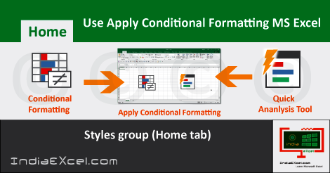
As we know that, the Styles group has the Conditional Formatting button. So, we’ll know How to Use Apply Conditional Formatting in a worksheet, in this post. This button has total Eight buttons. Some of them’re the Highlight Cell Rules button, the Data Bars button and the Icon Sets button etc; and so on.

Also, in one of the posts, we firstly got to know about the Conditional Formatting buttons. But, through this post, we’ll now know, how to use and apply them. Especially, the Conditional Formatting feature is quite captivating and attractive in terms of the functionality in Excel.

Because, the Conditional Formatting helps users to distinguish between the data in worksheet. In addition, also users can highlight necessary aspects in the data using these various buttons. So, to apply the Conditional Formatting in a cell or multiple cells, these steps’re required. We’re taking an example of some random numbers present in a column.

Use Apply Conditional Formatting MS Excel – continued

• First of all, select the Column, Row or the Range of Cells which have numbers.
• Then, go to the Highlight Cell Rules and select Greater Than button.
• A Greater than dialog show up.
• Now, type the number in the Text Box under Format cells that are GREATER THAN.
• Next, select the color from the Combo Box on the right side of the Text Box.
• And, finally click the OK button to Use and Apply the Conditional Formatting Rule.

Similarly, the other buttons such as the Less Than button or the Text that Contains button etc; and so on, functions on the same process. But, the New Rule button, the Clear Rules button and the Manage Rules button works slightly different.

Above all, also the Quick Analysis introduced in Microsoft Excel 2013 and Microsoft Excel 2016; helps to quickly and easily apply some of the types of Conditional Formatting rules. The Shortcut Key for the Quick Analysis tool is “Ctrl+Q“.

See Next Post: Understand Fill Handle worksheet Microsoft Excel 2016

Tags: Microsoft Excel Buttons