SumIf function of Math Trig functions in Microsoft Excel 2016
SumIf function Formulas tab MS Excel
Previous Post: Concatenate function of Text functions in Microsoft Excel 2016
Before we jump to know about this function in detail, let us understand few things. The SumIf function is very important in Microsoft Excel. Specifically, two functions i.e. “Sum” and “If” are combined together. It is part of the Math Trig functions of the Formulas tab.
Previously we got to know about the Concatenate function. It is also part of the Formulas tab in the Text functions. This function helps users to join multiple words from different cells. To know more about this function, kindly check the previous post.
SumIf function Formulas tab Excel 2016 – continued
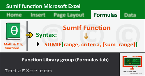
Especially, the SumIf functions helps to add numbers using an If condition. It means that, when the If condition becomes True, the addition of the numbers happens. So, the Syntax of the SumIf function is as follows,
Syntax: SUMIF(range, criteria, [sum_range])
First of all, the “Range” input parameter points to select the cells that users don’t want to sum. Obviously, this will be texts, words etc. But, that’s not the case each and every time depending upon the data. Therefore, it only depends on our own work, the type of results we want to get from the available data.
Further, the “Criteria” input is the expression, text or the number indicating the inside cells for addition. And, the “Sum_Range” input is the range of cells having the numbers, for the addition.
In order to understand about this function we’ll have to refer to an example. Suppose, we have a column having words Insurance, Loans, Mortgage etc. And, in the same adjacent column cells in front of each of these words we input following values:
SumIf function Math Trig functions MS Excel
For Insurance 21, Loans 32, Mortgage 45, Insurance 115, Mortgage 98, Loans 202. Alright, imagine a table of two columns of this type having this data. Now, on the right side we have a one more table of columns. In the first we have the same names as mentioned in the first line.
And, in the second adjacent column, we want the sum of the numbers according to these words. So, after applying the function syntax, we’ll have to select the first column for the “Range”. Then, select the first cell from the first column of the right side table, for the “Criteria” input.
Lastly, the input for the “Sum_Range” is the second column of the first table having the numbers. Select all the inputs as mentioned and then press Enter key. The sum for the Insurance word occurring two times, will result (21+115) i.e. 136. Likewise, then drag the Fill Handle, and the rest of words having the numbers will add up as well.
See Next Post: Add Cells with Text and Numbers Microsoft Excel 2016

Stay Connected
Connect with us on the following social media platforms.