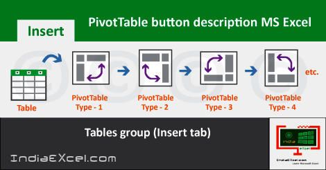
PivotTable button description of Tables group MS Excel

PivotTable button of Tables group Microsoft Excel

PivotTable button Tables group Microsoft Excel 2016

See Previous Post: Find Select buttons tools Editing group Microsoft Excel 2016

First of all, the Tables group is part of the Insert tab. And, in this post, the PivotTable button shall be discussed. So, this group has three buttons. Those are the Recommended PivotTables button, the Table button and the topic of this post.

Specifically, the PivotTable isn’t just an ordinary table. Especially, The PivotTable helps to ease the tasks quickly which’re performed within a Table. The creation of a table require components such as the Header Title, Columns, Rows and the Borders etc; and so on.

Let us assume, we’ve created a complete Table in Excel. And, our requirement is to swap the Header Row with the first Left Column. But, the data between the Row and Column cells should remain as it is.

PivotTable button of Tables group MS Excel – continued

So, for this we need some time, to perform the Cut or Copy operations; and also we’ll most probably use the Transpose button etc. There’s no doubt, we will able finally achieve this task, but what about the time spent to do the steps.

Therefore, the to get rid of all the lengthy steps, instead we should use the PivotTable button. And, after using this button, the task will get complete using a few steps.

• Firstly, select the table that has data in it.
• Then, click on PivotTable button.
• A Create PivotTable dialog box will show up.
• Next, click on the Select a table or range Radio/Option button.
• Click the OK button.

Now, the PivotTable Tools with Analyze and the Design tabs will show up; in the ribbon within a new worksheet. This confirms that we’ve successfully done the steps; and now the PivotTable Fields show up on the right side of the sheet.

PivotTable button of Tables group Excel 2016

Then, from this Window that has come up on the right; choose the fields one by one by putting a tick/check mark. Alternatively, we could drag and drop the fields into the boxes, which are present at the bottom.

They’re the Filters, the Columns, the Rows and the Values boxes. Most noteworthy, the fields that we select one by one are the Top Headers texts of the table. And, we can drag and drop them into any of the boxes. Because, it mainly depends upon our requirements that what type of new table we need.

Lastly, on the left side of the PivotTable Fields window; a new table has been created, from the same table that we initially selected. Also, if we change the fields locations in the boxes; the table also changes to a new one each time. So, finally we have our PivotTable now. And, that was all about, how to create new table types; from a existing table using the PivotTable button.

See Next Post: Add Pictures Insert Images worksheet Microsoft Excel 2016

Tags: Microsoft Excel Buttons