Microsoft Excel VLOOKUP vs INDEX MATCH: Definitive Guide for Data Analysts

Why INDEX MATCH Dominates Advanced Excel Spreadsheet Tips

Previous post: Troubleshooting MS Excel Clipboard Error: “We Couldn’t Free Up Space”

Unlocking Microsoft Excel Formulas for Better Efficiency

Are you tired of manually searching for specific data points in your massive spreadsheets? Microsoft Excel VLOOKUP vs INDEX MATCH Ultimate Guide is here for users in the United States and Worldwide; that face complex data management problem every single day. Fortunately, powerful Excel lookup functions exist to solve this tedious issue instantly. When you dive into Excel data analysis, you inevitably encounter the two most famous data retrieval tools: VLOOKUP and the highly dynamic INDEX MATCH combination.

While spreadsheet beginners usually start their journey with VLOOKUP, seasoned financial analysts fiercely debate which formula reigns supreme. This detailed comparison between the index match function and vlookup in microsoft excel will equip you with the knowledge to choose the perfect tool for your dynamic data lookup needs.

The Appeal and Limitations of VLOOKUP

VLOOKUP stands for “Vertical Lookup,” and it serves as the ultimate gateway to automated data retrieval. The formula simply searches for a specific value in the first column of your selected data table and returns a related value from another column in the exact same row. You only need four straightforward arguments to make it work, which explains why so many professionals rely on it for quick, static tasks. If you maintain simple inventory tracking sheets or basic employee directories, VLOOKUP does the job perfectly and saves you countless hours.

However, VLOOKUP possesses several frustrating limitations that frequently drive advanced users out of their mind in first place. First, it strictly searches from left to right. If you want to perform a left lookup in Excel, VLOOKUP instantly fails you. Your reference value must always sit securely in the far-left column of your selected table array. Second, VLOOKUP relies heavily on a hard-coded column index number. If you or a coworker insert or delete a column in your spreadsheet, VLOOKUP completely breaks. You then waste precious time manually fixing broken formulas across your entire workbook.

When you handle complex corporate datasets, you need a robust solution that never breaks. This is where INDEX Lookup Reference button functions of Function Library group Excel MATCH function steps in as the undisputed champion of Microsoft Excel formulas. Instead of acting as a single, rigid function, it combines two highly versatile formulas to create a dynamic data lookup powerhouse. The INDEX function returns the actual value of a cell located in a specific row and column, while the MATCH function accurately identifies the exact relative position of your lookup value. 

The benefits of combining these two powerful functions easily outshine VLOOKUP. Most importantly, INDEX MATCH looks in absolutely any direction—left, right, up, or down. It effortlessly solves the dreaded left lookup in Excel problem. Furthermore, because INDEX MATCH dynamically references actual column positions rather than fixed numeric values, you can freely insert, move, or delete columns without destroying your formulas. 

Choosing Your Ultimate Lookup Strategy

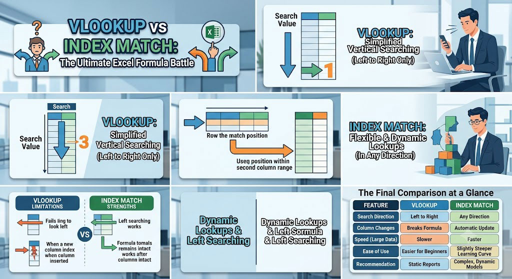
**Microsoft Excel VLOOKUP vs INDEX MATCH**

Ultimately, your specific project requirements dictate which formula you should implement. If you need a rapid, temporary fix for a small, unchanging data table, VLOOKUP remains incredibly useful. You can type it quickly and get your answer in mere seconds. Conversely, if you build professional business dashboards, manage extensive databases, or collaborate on frequently updated spreadsheets, you absolutely must adopt INDEX MATCH. Embracing these advanced Excel spreadsheet tips will drastically improve your workplace efficiency, eliminate costly manual errors, and elevate your skills!

Feature	VLOOKUP	INDEX MATCH
Search Direction	Left to Right only	Any Direction (Left, Right, Up, Down)
Column Changes	Breaks formula if columns are inserted/deleted	Automatically updates and remains intact
Speed (Large Data)	Slower, consumes more memory	Faster, highly efficient for large datasets
Ease of Use	Easier for beginners to learn	Slightly steeper learning curve
Best Used For	Quick, static reports and simple tables

Practical Example: U.S. Regional Sales Data Lookup

Suppose you manage a sales performance dataset for major U.S. market hubs:

Column A (State)	Column B (City)	Column C (Sales Rep)	Column D (Quarterly Revenue)
California	Los Angeles	Sarah Jenkins	$142,500
Texas	Houston	Marcus Vance	$118,200
New York	New York City	Elena Rostova	$165,000
Florida	Miami	David Miller	$98,400

Scenario 1: standard Right-Side Lookup (VLOOKUP Works)

Goal: Find the Quarterly Revenue for the Texas region.

Because the lookup column (State) is on the far-left (Column A) and the target column (Revenue) is to its right (Column D), VLOOKUP works without issues:

\text{=VLOOKUP("Texas", A2:D5, 4, FALSE)}

Result: $118,200
Why it works: VLOOKUP searches Column A for “Texas” and returns the value from the 4th column in that row.

Scenario 2: Left-Side Lookup (VLOOKUP Fails, INDEX MATCH Succeeds)

Goal: Retrieve the State based on the Sales Rep name (“Elena Rostova”).

Here, your lookup criteria is in Column C, but your desired result (State) is in Column A (to the left).

VLOOKUP Attempt: Fails because VLOOKUP cannot search to the left of its lookup column.
INDEX MATCH Solution:

\text{=INDEX(A2:A5, MATCH("Elena Rostova", C2:C5, 0))}

How it works:
1. MATCH("Elena Rostova", C2:C5, 0) finds “Elena Rostova” in row 3 of the range C2:C5.
2. INDEX(A2:A5, 3) fetches the value from row 3 of the target range A2:A5.
Result: New York

Scenario 3: Column Insertion / Spreadsheet Editing

Goal: Keep your Revenue lookup intact if a new column (e.g., “Region Code”) is inserted between City and Sales Rep.

VLOOKUP Problem: If you insert a column, Revenue shifts from column 4 to column 5. The fixed col_index_num of 4 in =VLOOKUP("Texas", A2:D5, 4, FALSE) will now return the wrong data column or break.
INDEX MATCH Solution:

\text{=INDEX(D2:D5, MATCH("Texas", A2:A5, 0))}

Why it succeeds: Because D2:D5 and A2:A5 are direct range references, Excel automatically updates the range to E2:E5 when you insert a column, ensuring your formula never breaks!

This practical example directly demonstrates how INDEX MATCH handles reverse lookups and column shifts in large business datasets.

For a step-by-step video breakdown of lookup speed and performance tricks, check out this tutorial on INDEX + MATCH vs VLOOKUP: Faster Sales Lookup, which shows how professionals apply these exact formulas to real sales datasets.

See Next Post: Beyond the Formula Bar: How Agentic AI and Python are Reimagining Excel

Tags: Microsoft Excel Functions, Microsoft Excel Tips

About the Author

After working on Microsoft Excel for so many years, now its time to share & spread my Experience and Knowledge, which I have gained on Excel with the world. Myself, Piyush Kr. Pandey is an Excel enthusiast and founder of IndiaExcel.com (Learn Microsoft Excel), a website since 2016. Kindly, Subscribe our blog email newsletters for daily vital and essential informative posts on Microsoft Excel. Email: indiaexcelblog@gmail.com More from this author »