How to Create a Pivot Table in Excel (Step-by-Step Data Summary)

Previous post: How to Create Charts in Excel (The Complete Visual Reporting Guide)

Imagine your boss hands you a corporate sales spreadsheet with over 5,000 individual transactional rows. They want you to find out the total sales generated by each product across different regional branches by the end of the day.

If you try to manually sort, filter, and write hundreds of SUMIF formulas, you will waste hours. Instead, you can use the most powerful tool in the Microsoft Excel arsenal: Pivot Tables.

Located right inside the Tables group on your Insert tab, Pivot Tables allow you to summarize, analyze, and slice massive datasets in just a few clicks without writing a single line of code.

In this step-by-step tutorial, you will learn exactly how to initialize a Pivot Table, organize your data fields, and avoid the common traps that break your reports.

Step 1: Finding the Tables Group on the Insert Tab

To launch your data summary report, look at the very beginning of your primary toolbar panel:

1. Open your active spreadsheet containing your data rows.
2. Click on the Insert tab on the main Ribbon interface.
3. Look all the way to the far-left side to locate the Tables group.
4. You will see three distinct foundational buttons: PivotTable, Recommended PivotTables, and Table.

Step 2: Setting Up Your First Pivot Table

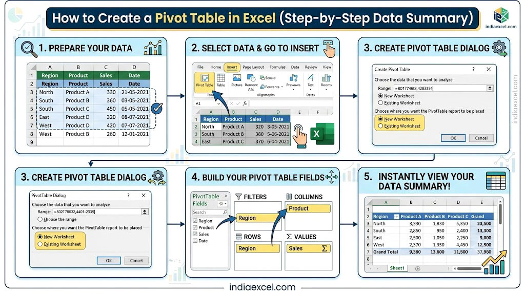
Before clicking, ensure your source table has clean column headers (e.g., Date, Employee, Region, Sales and zero completely empty rows.

1. Click any single active cell inside your data block.
2. Navigate to the Insert tab and click the PivotTable button.
3. A popup window titled PivotTable from table or range will appear. Excel will automatically highlight your entire contiguous data range.
4. Choose New Worksheet as the destination where you want the report to sit, and click OK.

Step 3: Mastering the 4 Pivot Table Quadrants

Once clicked, Excel will open a blank summary canvas on a new sheet and unlock the PivotTable Fields sidebar panel on the right. To build your report, simply click and drag your column headers into these four structural quadrants:

• 1. Rows: Drag the items you want to list vertically down the left side (e.g., drag Product Names here).
• 2. Columns: Drag the items you want to display horizontally across the top (e.g., drag Regions here to compare markets side-by-side).
• 3. Values: Drag the numerical fields you want to calculate here (e.g., drag Sales Revenue here). Excel will instantly total up all the numbers automatically.
• 4. Filters: Drag any field here if you want an overarching drop-down menu at the top to isolate specific data lines (e.g., drag Year here).

💡 Pro Tip: The “Recommended PivotTables” Shortcut

If you are a beginner and looking at a blank canvas feels intimidating, go back to the Insert Tab > Tables Group and click Recommended PivotTables.

Microsoft Excel’s AI engine will instantly scan your data patterns and generate a structural gallery of 5 or 6 ideal layout previews (such as Sum of Sales by Region or Count of Orders by Category). Select the layout that matches your goal and click OK to build it instantly.

🛠️ Troubleshooting: Common Pivot Table Errors

1. Error: “The PivotTable field name is not valid”

This is the most common error message users face when clicking the Insert button. It happens because one of your source data columns has a completely blank header cell.

• The Quick Fix: Go back to your main data sheet, check row 1 entirely, make sure every single column has a clear text name, and re-insert the table.

2. The Total Values are Showing “Count” Instead of “Sum”

If you drag your revenue column into the Values box and Excel shows you the total number of transactions (e.g., 45) instead of the actual dollar amount (e.g., $120,000), your source data contains text letters mixed with numbers.

• The Quick Fix: Right-click any number inside your Pivot Table values column, select Summarize Values By, and switch the checkmark from Count to Sum.

❓ Frequently Asked Questions (FAQ)

Why is my Pivot Table not updating when I change my source numbers?

Unlike standard formulas, Pivot Tables do not recalculate automatically when you edit numbers in your core rows. To fetch the updated data, right-click anywhere inside your Pivot Table layout and click the Refresh button icon.

See Next Post: How to Use Data Validation in Excel (Create Dropdowns & Restrict Inputs)